Nov. 3, 2025 – In the investment realm, the Sharpe ratio is widely regarded as one of the most impactful evaluation metrics for calculating risk-adjusted returns. Created in 1966 by American economist and Nobel laureate William Forsyth Sharpe, this quantitative formula—originally dubbed the “reward-to-variability ratio” effectively compares the excess return of an investment to its volatility to help determine if the gains justify the associated risk.

By the Numbers

The Sharpe ratio is a straightforward formula comprising three key inputs:

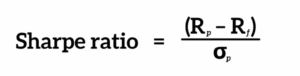
R_p = return of portfolio. This either represents an asset’s historical or forecasted data over a given period as a percentage of an investment. For example, if an equity averaged 10% annual returns over its lifetime, then R_p = 10. But for an exchange-traded fund with a 5-year, 30% return, the R_p = 30. In either case, this value combines an investment’s capital gains (or losses) and any dividends.

R_f = risk-free rate. This benchmark, which expresses the gains an investor would earn on an asset with virtually no risk, commonly uses U.S. Treasury bills because these securities rarely default. In most practical applications the 3-month Treasury bill is used because it is liquid, short term and reflects a near-risk-free return for most investment horizons. While some practitioners use longer-term or matching rates to the timeframe of the return of portfolio, the most common choice is the 3-month T-bill for consistency.

σ_p = standard deviation. The denominator in the equation measures volatility by identifying the extent to which the price of the asset fluctuates over the same time period. Always expressed as a positive number, the standard deviation represents both performance upswings and downswings, where higher numbers correlate to higher price volatility.

By plugging these three values into the formula, assessments can be made based on the output. A higher Sharpe ratio generally indicates that an investment is providing more return for the risk taken.

A Tale of Two Investments

To see just how the Sharpe ratio can help guide investors, consider the following examples:

Example 1: Imagine an investor who owns a single stock that’s historically had a 15% return over a certain period, where the risk-free rate of a Treasury bond is 3%, and the standard deviation is 8%. Plugging those values into the Sharpe formula would be: (15%-3%)/8% = 1.5. This means the asset’s excess return above the risk-free rate is 1.5 times its standard deviation, signaling a modestly favorable risk-adjusted return.

Example 2: Now consider a fund with a 15% annual return, a risk-free rate of 3%, and a standard deviation of 12%. The Sharpe ratio would be calculated as (15%-3%)/12% = 1.0. This indicates that for every unit of risk taken, the fund generated 1.0 units of excess return.

Comparing these two examples, the single stock investment in example one offers better return per unit of risk.

Practical Use

While the Sharpe ratio contextualizes the relative risk of an investment compared to its return profile, financial professionals are free to deploy this metric however they see fit. Pointedly, some might decline to engage in an investment with a high Sharpe ratio because even if the potential gains are favorable on a risk-adjusted basis, they may not be comfortable with that risk level. For example, a stock returning 200% over the past five years, with a 4% risk-free rate and 50% standard deviation, carries a Sharpe ratio of 3.92. While this may seem attractive on its face, some may be hesitant to allocate their investment account to an asset that might give up half of its value when they could instead conservatively invest in a 4%-yielding Treasury bond.¹

Built-in Versatility

One reason the Sharpe ratio is so widely utilized is because it affords the option of either using historical returns or forecasted returns in the R_p inputs, allowing the metrics to be tailored according to individual preferences. Forward-looking individuals can use future performance to help decide where to allocate capital. Contrarily, historical returns let financial professionals backtest strategies to provide a keen understanding of how they performed, letting them compare how different strategies stack up—whether it’s a value-driven, momentum or macro-driven approach.

Sharpe Ratio Limitations

While the Sharpe ratio is a helpful benchmark, it should be considered carefully alongside other factors such as time period, data frequency, strategy and individual investment goals. Since it is based on price variability inputs, Sharpe ratios don’t account for other costs or risks such as transaction costs, management fees, off-market valuations or leveraged assets. For these reasons, Sharpe enables comparison across various asset classes, including alternatives, by standardizing risk and return but illiquidity and valuation frequency create limitations of its use.

Furthermore, standard deviation assumes there’s an equal distribution of returns, which is only true in theory—not in practice. For this reason, it’s vital to understand how the ratio has been calculated and to overlay the Sharpe metric with a company’s broader financials, including balance sheet strength, profitability and strategic positioning. Even with these limitations, the Sharpe ratio can be used for any type of investment, alongside other metrics for portfolio construction.

Conclusion

Strategically considered, Sharpe ratios can be an invaluable tool to help assess risk-adjusted returns. But since past or forecasted performance is not a guarantee of future results, it’s vital for investment professionals to conduct robust due diligence to maximize long-term profit potential.

¹ Lauren Perez and Jake Safane, “Understanding the Sharpe ratio: An explainer for investors,” Business Insider, April 22, 2025.

CSC-1125-4058145-INV